First steps with EPCY

EPCY is implemented in python3 and allows to perform predictive analyses using bash command line.

If it’s not already done, you need to install EPCY

pip install epcy
epcy -h

Input files

EPCY is designed to work on several quantitative data (like genes expression), provided that this data is normalized, that is quantitative values for each genes (features) need to be comparable between each samples. For RNA-seq data, TPM, FPKM or even counts per million reads (CPM) values would be appropriate (normalization per transcript length is not critical since we will be comparing quantities between samples, not within samples).

To run EPCY, you need two tabulated files, as input:

• A matrix of quantitative data, normalized for each samples (in columns) with an ID column to identify each genes (features), in first.

Example of a quantitative matrix

id	Sample1	…	SampleX
Gene1	10	…	20
…	…	…	…
GeneY	12	…	16

• A design table which describes the parameters or conditions on which to perform the analyses. This table is composed of a first column Sample, followed by at least one column which describes each sample for each parameter. A new column is needed for each parameter. For a gene knock-out experiment for instance, a column would indicate which samples are wild-type and which is knock-out.

Example of a design table

sample	Condition	Knockout_exp	Gender
Sample1	Query	KO	F
…	…	…	…
SampleX	Ref	WT	M

Download input files

For this tutorial, we propose to download a part of the Leucegene cohort composed by 88 Acute Myeloid Leukemia (AML) individual samples. To reduce the execution time, we are going to only analyze coding genes (19,892 genes). These input files are available in a specific git repo named epcy_tuto, and can be downloaded using git:

git clone git@github.com:iric-soft/epcy_tuto.git
cd epcy_tuto/data/leucegene

If you examine the design.txt file, you can see that an AML column is used to classify each sample into one of these 3 subtypes of AML: t15_17, inv16 and other. These refer to samples that show either a chromosome 15-17 translocation, a chromosome 16 inversion or other defect respectively.

design.txt

Sample	AML
01H001	Other
01H002	t15_17
…	…
13H120	inv16
…	…
14H133	t15_17

We will start by comparing t15_17 samples versus all other samples (inv16 and other). On a macbook pro 2 GHz Dual-Core Intel Core i5, this analysis takes 10 min, using 4 thread.

Run your first EPCY analysis

EPCY is divided into severals tools, which can be listed using:

epcy -h

Among all these tools, epcy pred is the one which allows to run a default comparative predictive analysis. In our current case, we would write:

epcy pred --log -t 4 -m cpm.tsv  -d design.txt --condition AML --query t15_17 -o ./29_t15_17_vs_59/
# Or if you only want compare versus inv16 subgroup
epcy pred --log -t 4 -m cpm.tsv  -d design.txt --condition AML --query t15_17 --ref inv16 -o ./29_t15_17_vs_27_inv16/

where:

• --log: specifies that quantitative data needs to to be log transformed before being analyzed.

• -t 4: allows to use 4 threads for the analysis.

• -m cpm.tsv: specifies the quantitative matrix file.

• -d design.txt: specifies the design table.

• --condition AML: determines the condition column we want use.

• --query t15_17: specifies which subgroup of AML samples we want to compare to all the other.

• -o ./29_t15_17_vs_59/: specifies the output directory.

More information can be found, using epcy pred -h.

If everything is correct, the analysis will complete by displaying the following output:

15:43:02: Read design and matrix features
15:43:04: 181 features with sum==0 have been removed.
15:43:04: Start epcy analysis of 19766 features
15:52:22: Save epcy results
15:52:22: End

Results

predictive_capability.tsv is the main output of an EPCY analysis. It is a tabulated file which contains the evaluation of each genes (features) for its predictive value, using 9 columns:

• id: the id of each gene (feature).

• l2fc: log2 fold change.

• kernel_mcc: Matthews Correlation Coefficient (MCC) compute by a predictor using KDE.

• kernel_mcc_low: lower bound of the confidence interval (90%).

• kernel_mcc_high: upper bound of the confidence interval (90%).

• mean_log2_query: average of log transformed values of this feature for samples in the subgroup of interest defined using the –query parameter.

• mean_log2_ref: average of log transformed values of this feature for samples in the reference group.

• bw_query: estimated bandwidth used by KDE, to calculate the density of query samples.

• bw_ref: estimated bandwidth used by KDE, to calculate the density of ref samples.

Genes (features) with the highest kernel_mcc values correspond to the most prodictive ones. The file may then be sorted on that column to obtain the following:

./29_t15_17_vs_59/predictive_capability.tsv ordered on kernel_mcc

id	l2fc	kernel_mcc	kernel_mcc_low	kernel_mcc_high	mean_query	mean_ref	bw_query	bw_ref
ENSG00000183570.16	3.97	0.98	0.95	1	4.84	0.87	0.24	0.42
ENSG00000168004.9	3.75	0.97	0.97	0.97	4.00	0.24	0.28	0.10
ENSG00000089820.15	-4.25	0.97	0.62	0.97	4.21	8.47	0.34	0.23
…	…	…	…	…	…	…	…	…

Note: Since EPCY uses some random steps in its implementation, you may observe small variations in your results. The argument -- randomseed 42 can be used to obtain the exact same results (see Reproductibility section).

Quality control

EPCY needs to have enough data to train the KDE classifier and evaluate the predictive capability of each gene (feature) accurately. Without enough samples, EPCY will overfit and return a large number of negative MCC.

Unfortunately, it is a priori difficult to detemine a lower bound for the number samples needed, as this number will depend on the dataset analyzed. However, EPCY provides some quality control tools (epcy qc), to verify if there is overfitting or not, by checking the distribution of MCC and bandwidth.

Using epcy qc, we can plot two quality control figures, as follow:

epcy qc -p ./29_t15_17_vs_59/predictive_capability.tsv -o ./29_t15_17_vs_59/qc

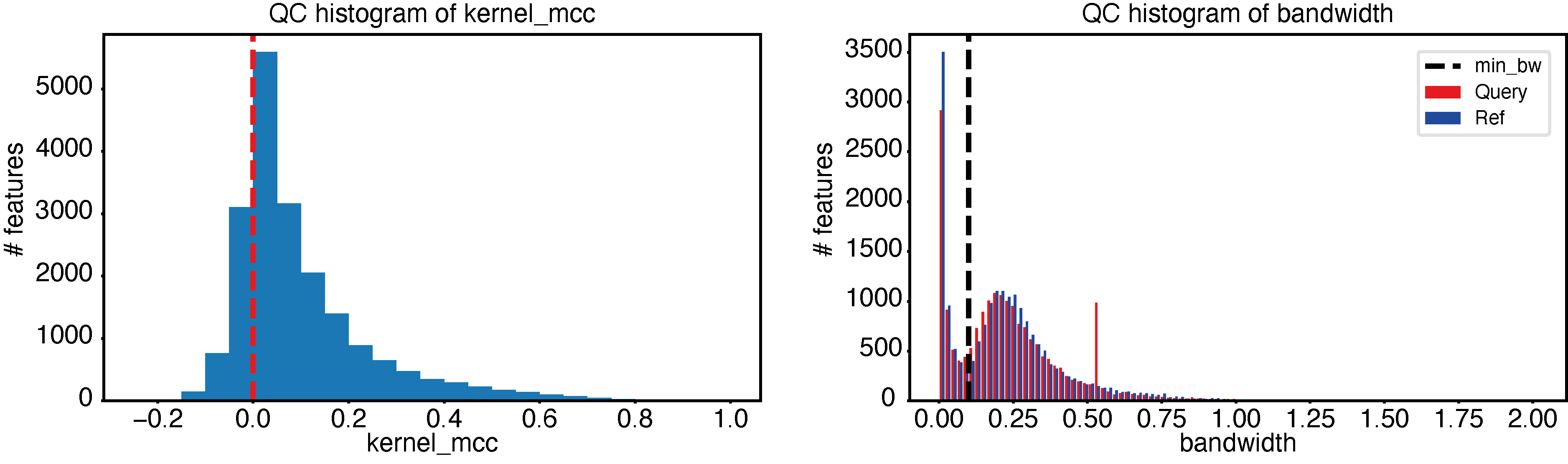
We can see in these graphs that quality is good, since:

• Most negative MCC, are close to 0.

• The minimum bandwidth (default 0.1), avoids learning from variations represented by the first mode of the distribution.

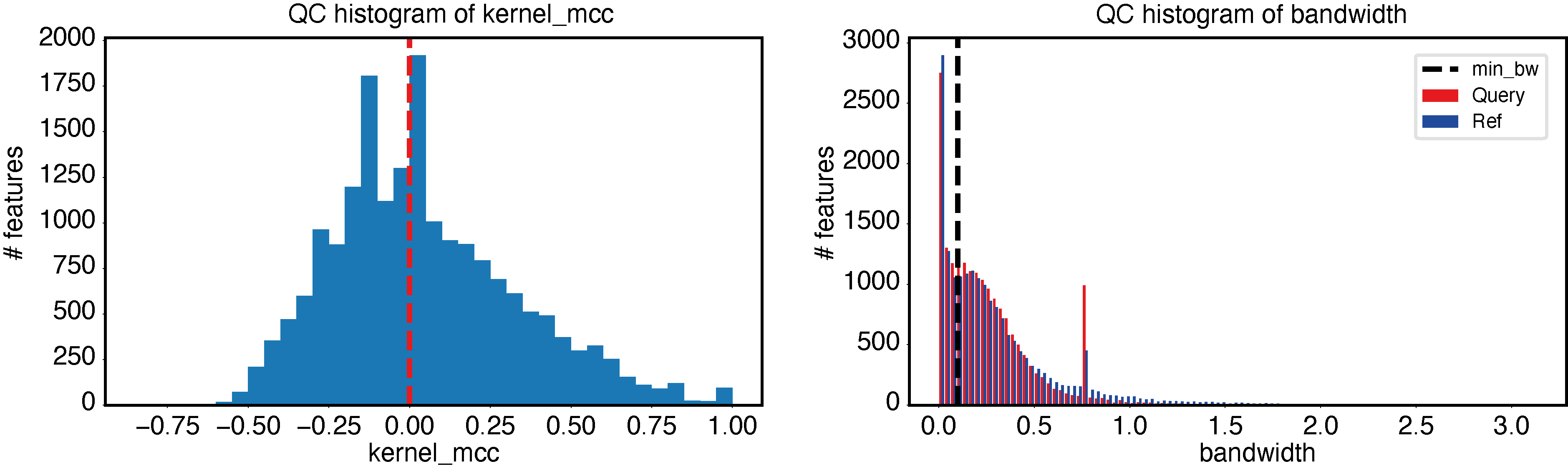
An example of bad quality control results can be made by simulating a dataset that is too small, as follows:

epcy pred --log -t 4 -m cpm.tsv  -d design_10_samples.txt --condition AML --query t15_17 -o ./5_t15_17_vs_5/
epcy qc -p ./5_t15_17_vs_5/predictive_capability.tsv -o ./5_t15_17_vs_5/qc

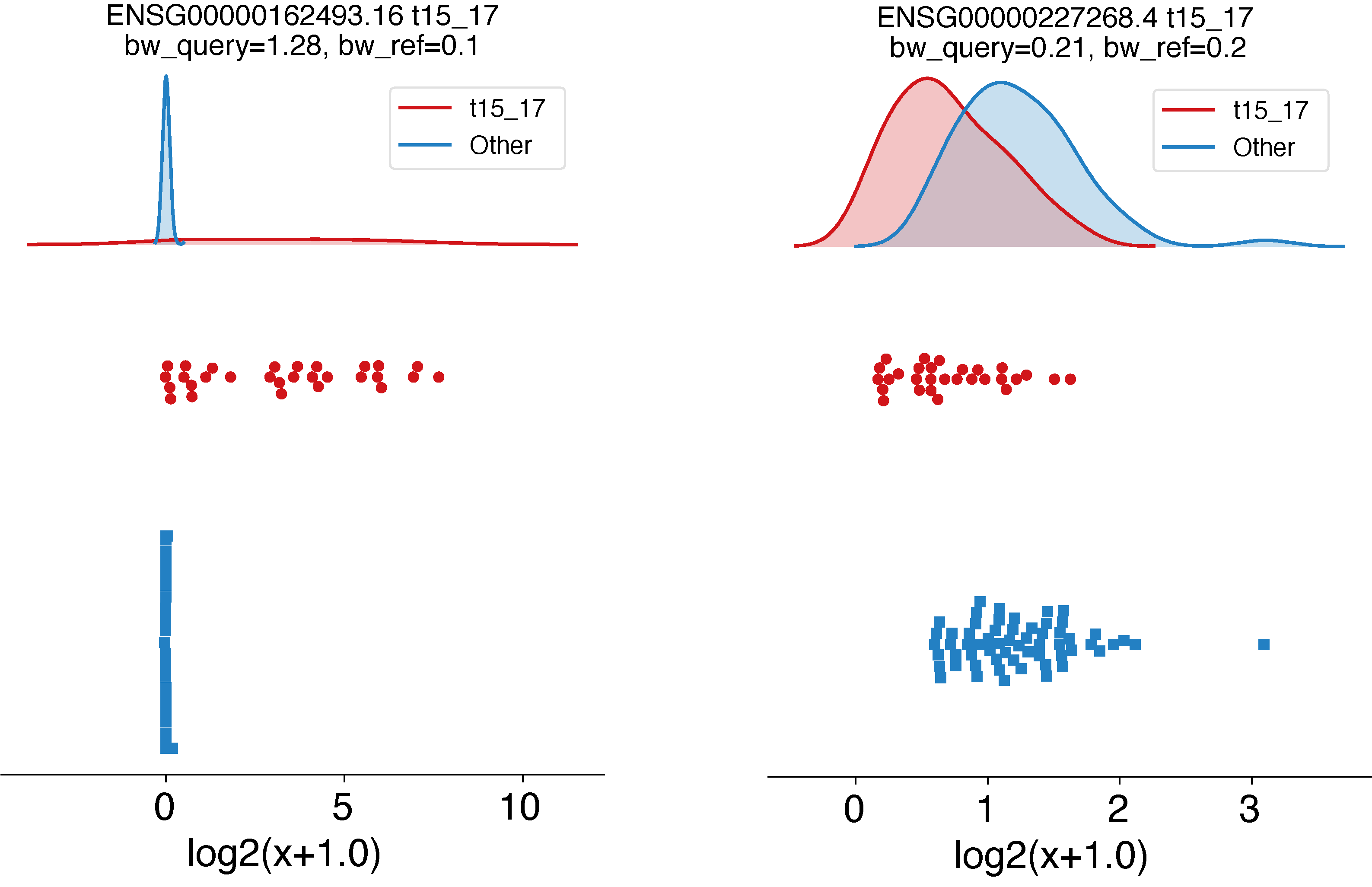
Plot a KDE trained on gene expression

EPCY also provides some visual tools, which can help with the exploration of your dataset. Using epcy profile, we can plot the gene expression distribution, along with the trained KDE classifier that represents each condition.

# ENSG00000162493.16 (PDPN, MCC=0.87), ENSG00000227268.4 (KLLN, MCC=0.33)
epcy profile --log -m cpm.tsv -d design.txt --condition AML --query t15_17 -o ./29_t15_17_vs_59/figures/ --ids ENSG00000162493.16 ENSG00000227268.4

Reproducibility

EPCY draws a random value to assign a class according to probabilities learned by the KDE classifier, to fill a contingency table (see algorithm section). This means that different runs of EPCY can produce different results.

However, the output of EPCY is relatively stable, since each predictive score returned is already a mean of several predictive score calculations (by default 100), which are performed to minimize variance between runs. Nevertheless, different runs might show small variations. To ensure reproducibility, we add a parameter to specify the seed of the random number generator, using --randomseed.

Here is an example on the dataset used for the tutorial (see, How to use EPCY).

epcy pred --randomseed 42 --log -t 4 -m cpm.tsv  -d design.txt --condition AML --query inv16 -o ./27_inv16_vs_61/

Some details on the design table

As mentioned before, the design.txt file classifies samples in 3 different subtypes (t15_17, inv16 and other). Similarly as we did for t15_17, we can analyse inv16 samples vs all others samples (t15_17 and other), using the command below:

epcy pred --log -t 4 -m cpm.tsv  -d design.txt --condition AML --query inv16 -o ./27_inv16_vs_61/

Moreover, it is possible to add more columns in design.txt, each one representing conditions you want to compare. Indeed, with the design table given as example (in introduction), we could perform an analysis on Gender, using --condition Gender --query M -o ./gender.

Also, if some annotations are unknown for some samples, we can remove these samples from the analysis by using None in the corresponding cell.

Example where the AML subtype of sampleX is unknown and needs to be removed from the analysis.

Sample	AML	Gender
Sample1	t15_17	M
…	…	…
SampleX	None	F

With all these variations, you should be able to perform any number of comparisons using a unique design file, or by creating a different design file for each comparison.